
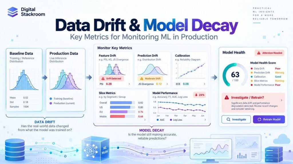
A machine learning model can remain completely unchanged in production while its predictions gradually become less useful.
The code did not break.
The endpoint is healthy.
Latency is normal.
There are no exceptions in the logs.
Yet the model that performed well six months ago is now making noticeably worse decisions.
This is one of the uncomfortable realities of production machine learning: a model is deployed into an environment that keeps changing after training ends.
Customers change.
Products change.
Marketing campaigns attract different populations.
Economic conditions move.
Upstream pipelines are rewritten.
Sensors are replaced.
Fraud strategies evolve.
Business policies change.
The statistical relationships the model learned may eventually stop describing the world in which the model is being used.
This is where data-drift and model-performance monitoring become essential.
But there is an important distinction that is frequently lost in monitoring dashboards:
Data drift is not the same thing as model decay.
A feature distribution can change significantly while model performance remains stable.
A model can also lose accuracy even when the marginal feature distributions look almost unchanged.
In this guide, we will build a practical monitoring framework for production machine learning and examine:
- training-serving skew
- feature drift
- categorical and numerical drift
- prediction drift
- concept drift
- model decay
- Kolmogorov-Smirnov statistics
- Wasserstein distance
- Jensen-Shannon distance
- Population Stability Index
- classification performance
- calibration
- delayed labels
- segment-level monitoring
- seasonal baselines
- alert design
- retraining decisions
We will also build a small Python lab that simulates a model moving from a stable validation population into a changed production population.
The goal is not to create a single “drift score.”
The goal is to answer a much more useful operational question:
Has something changed enough to threaten the model, and if so, what should we investigate next?
Table of Contents
The Production Problem: Models Age Even When Code Does Not
Imagine a credit-risk classifier trained in January.
At training time, the population looked like this:
Average customer age:      41
Average annual income:     $61,000
Primary region:            North
Positive outcome rate:     18%
Six months later:
Average customer age:      37
Average annual income:     $68,000
Primary region:            South
Positive outcome rate:     26%
Several things may now be different.
The input population changed.
The target rate changed.
The relationship between income and default may have changed.
The model may still rank customers correctly.
Or it may not.
Looking at only one metric cannot tell us which situation we are in.
A useful monitoring architecture therefore separates several kinds of change.
Data Drift, Concept Drift, and Model Decay Are Different Problems
These terms are sometimes used interchangeably, but they describe different things.
Training-Serving Skew
Training-serving skew occurs when the data seen during inference differs from the distribution the model saw during training or validation.
Conceptually:
Training Distribution
        ↓

P_train(X)

        ≠

P_production(X)
This can be caused by genuine user-population change, but it can also indicate an engineering problem.
For example:
Training:
annual_income = dollars

Production:
annual_income = cents
A drift detector would see a dramatic shift.
But the root cause is a data-pipeline defect, not changing customer behavior.
This is why drift monitoring should sit beside data-quality monitoring rather than replace it.
If you are building those upstream validation gates, the Digital Stackroom guide on Automating Data Validation Pipelines with SQL Assertions covers schema, null, uniqueness, referential-integrity, freshness, and volume checks that should happen before model-drift analysis.
Feature Drift
Feature drift means the statistical distribution of one or more input features has changed over time.
Mathematically:
P_reference(X)
       ≠
P_current(X)
For example:
Reference:

customer_age
mean = 41

Current:

customer_age
mean = 35
Feature drift can affect model performance, but it does not guarantee that performance deteriorated.
Prediction Drift
Prediction drift means the model’s output distribution changes.
For a classifier:
Reference predicted probabilities:

0.05
0.10
0.12
0.24
0.81
...

Current predicted probabilities:

0.35
0.42
0.57
0.61
0.90
...
Or perhaps the percentage of cases classified as positive changes from:
18%to:
31%Prediction drift is an important operational signal.
But it still does not prove that the model became less accurate.
The population itself may genuinely have changed.
Target Drift
Target drift occurs when the distribution of the outcome changes.
For example:
Training fraud rate:    1.2%
Current fraud rate:     2.8%
This can materially change operating conditions even if feature distributions remain fairly stable.
Target drift is observable only when ground-truth labels eventually become available.
Concept Drift
Concept drift is more fundamental.
It means the relationship between the features and target has changed.
Conceptually:
P_reference(Y | X)
        ≠
P_current(Y | X)
Suppose income was once a strong predictor of loan default.
After a major economic event, customers with identical income profiles may behave differently.
The same input no longer implies the same probability of the target.
This is concept drift.
Looking only at:
P(X)cannot reliably detect it.
You normally need labels or another meaningful outcome signal to establish that the relationship between inputs and outcomes has changed.
Model Decay
Model decay is the operational outcome we ultimately care about.
It means the model’s real-world predictive performance has deteriorated relative to an accepted baseline.
For a classifier:
ROC-AUC
0.87 → 0.79
or:
Recall
0.76 → 0.61
For a regression model:
MAE
4.2 → 7.1
The exact metric depends on the business problem.
The key principle is:
Drift
≠
Decay
Drift is evidence that the world has changed.
Decay is evidence that the model is no longer performing as expected.
A Practical Monitoring Architecture
A production monitoring system should observe more than model accuracy.
I generally think of it as several layers.
                         PRODUCTION REQUESTS

                                ↓

                     ┌─────────────────────┐
                     │ Data Quality Checks │
                     │ Schema / Missingness│
                     └──────────┬──────────┘
                                ↓
                     ┌─────────────────────┐
                     │ Feature Drift       │
                     │ Numerical / Category│
                     └──────────┬──────────┘
                                ↓
                     ┌─────────────────────┐
                     │ Model Predictions   │
                     │ Score Distribution  │
                     └──────────┬──────────┘
                                ↓
                     ┌─────────────────────┐
                     │ Business Outcomes   │
                     │ Labels Arrive Later │
                     └──────────┬──────────┘
                                ↓
                     ┌─────────────────────┐
                     │ Performance Metrics │
                     │ AUC / F1 / MAE etc. │
                     └──────────┬──────────┘
                                ↓
                     ┌─────────────────────┐
                     │ Slice Analysis      │
                     │ Region / Segment    │
                     └──────────┬──────────┘
                                ↓
                     ┌─────────────────────┐
                     │ Alert / RCA /       │
                     │ Retraining Decision │
                     └─────────────────────┘
This design lets us answer two different questions:
Did the production environment change?

and

Did that change actually damage model performance?
Step 1: Create a Reproducible Monitoring Lab
We will build a binary-classification example.
Install the required libraries:
pip install -U numpy pandas scipy scikit-learnImport them:
import numpy as np
import pandas as pd

from scipy.spatial.distance import jensenshannon
from scipy.stats import ks_2samp, wasserstein_distance

from sklearn.compose import ColumnTransformer
from sklearn.linear_model import LogisticRegression
from sklearn.metrics import (
    average_precision_score,
    brier_score_loss,
    f1_score,
    log_loss,
    precision_score,
    recall_score,
    roc_auc_score,
)
from sklearn.model_selection import train_test_split
from sklearn.pipeline import Pipeline
from sklearn.preprocessing import OneHotEncoder, StandardScaler
For this lab we will generate fictional customer data.
Using synthetic data makes the notebook reproducible without exposing real customer information.
If you need realistic tabular test data for staging environments, see Synthetic Tabular Data Generation with SDV and CTGAN. The important distinction is that synthetic datasets can help test pipelines, but they do not automatically prove real production behavior.
Step 2: Generate a Reference Population
Create a sigmoid helper:
def sigmoid(x):
    return 1.0 / (1.0 + np.exp(-x))
Now generate a population.
def make_customer_batch(
    n: int,
    rng: np.random.Generator,
    age_shift: float = 0.0,
    income_scale: float = 1.0,
    region_probs=(0.45, 0.35, 0.20),
    concept_version: int = 1,
) -> pd.DataFrame:

    age = np.clip(
        rng.normal(
            loc=40 + age_shift,
            scale=10,
            size=n,
        ),
        18,
        80,
    )

    income = rng.lognormal(
        mean=np.log(60_000 * income_scale),
        sigma=0.35,
        size=n,
    )

    tenure = np.clip(
        rng.gamma(
            shape=2.5,
            scale=2.0,
            size=n,
        ),
        0,
        25,
    )

    region = rng.choice(
        ["North", "South", "West"],
        size=n,
        p=region_probs,
    )

    age_z = (age - 40) / 10

    income_z = (
        np.log(income)
        - np.log(60_000)
    ) / 0.35

    tenure_z = (
        tenure - 5
    ) / 4

    region_effect = np.select(
        [
            region == "North",
            region == "South",
            region == "West",
        ],
        [
            0.25,
            -0.10,
            0.05,
        ],
        default=0.0,
    )

    if concept_version == 1:

        logit = (
            -1.4
            + 0.55 * age_z
            + 0.70 * income_z
            + 0.30 * tenure_z
            + region_effect
        )

    elif concept_version == 2:

        # Deliberately change the relationship
        # between features and outcome.
        logit = (
            -1.2
            + 0.15 * age_z
            + 0.20 * income_z
            + 0.55 * tenure_z
            - region_effect
        )

    else:
        raise ValueError(
            "Unsupported concept_version."
        )

    probability = sigmoid(logit)

    label = rng.binomial(
        n=1,
        p=probability,
        size=n,
    )

    return pd.DataFrame({
        "age": age,
        "income": income,
        "tenure": tenure,
        "region": region,
        "label": label,
    })
Create the original population.
rng = np.random.default_rng(42)

reference = make_customer_batch(
    n=12_000,
    rng=rng,
)
Split it into training and a stable monitoring baseline.
train_df, baseline_df = (
    train_test_split(
        reference,
        test_size=0.33,
        random_state=42,
        stratify=reference["label"],
    )
)
The important decision here is that we do not evaluate production decay against training performance.
Training metrics are usually optimistic.
A better baseline is:
- holdout validation data
- out-of-time validation
- or a known-good production period
depending on the application.
Step 3: Create a Changed Production Population
Now simulate a later production period.
current_df = make_customer_batch(
    n=4_000,
    rng=rng,
    age_shift=-3.0,
    income_scale=1.10,
    region_probs=(
        0.25,
        0.55,
        0.20,
    ),
    concept_version=2,
)
Several things changed deliberately:
Age distribution changed
Income distribution changed
Regional mix changed
Feature/target relationship changed
This gives us both:
covariate drift
+
concept drift
The lab is intentionally designed to demonstrate the distinction.
It should not be interpreted as a benchmark of expected drift magnitude.
Step 4: Train the Model
Define features:
numeric_features = [
    "age",
    "income",
    "tenure",
]

categorical_features = [
    "region",
]
Create preprocessing:
preprocessor = ColumnTransformer(
    transformers=[
        (
            "numeric",
            StandardScaler(),
            numeric_features,
        ),
        (
            "categorical",
            OneHotEncoder(
                handle_unknown="ignore"
            ),
            categorical_features,
        ),
    ]
)
Build the model pipeline:
model = Pipeline(
    steps=[
        (
            "preprocess",
            preprocessor,
        ),
        (
            "classifier",
            LogisticRegression(
                max_iter=1000
            ),
        ),
    ]
)
Train:
X_train = train_df[
    numeric_features
    + categorical_features
]

y_train = train_df["label"]

model.fit(
    X_train,
    y_train,
)
Generate baseline predictions:
X_baseline = baseline_df[
    numeric_features
    + categorical_features
]

baseline_df = baseline_df.copy()

baseline_df["score"] = (
    model.predict_proba(
        X_baseline
    )[:, 1]
)
Generate current predictions:
X_current = current_df[
    numeric_features
    + categorical_features
]

current_df = current_df.copy()

current_df["score"] = (
    model.predict_proba(
        X_current
    )[:, 1]
)
Now we have:
Reference inputs
Reference labels
Reference model scores

Current inputs
Current labels
Current model scores
That gives us everything needed to monitor both drift and decay.
Step 5: Monitor Data Quality Before Measuring Drift
Before comparing distributions, check whether the data itself is valid.
For each feature, I would normally monitor:
| Data-quality signal | Example |
|---|---|
| Missing rate | income NULL rate |
| Schema/type | numeric field becomes string |
| Range | age = -300 |
| Cardinality | region suddenly has 800 values |
| Unknown categories | unexpected source values |
| Volume | 1M rows drops to 10K |
| Freshness | feed stops updating |
| Duplicates | repeated prediction IDs |
A major distribution shift caused by a malformed pipeline should not immediately trigger model retraining.
It should trigger a data incident.
This is the first reason I keep data validation and statistical drift as separate monitoring layers.
Step 6: Monitor Numerical Features With the KS Statistic
The two-sample Kolmogorov-Smirnov test compares the empirical cumulative distributions of two continuous samples.
SciPy exposes it through:
ks_2samp()Create a helper.
def ks_drift(
    reference: pd.Series,
    current: pd.Series,
) -> dict:

    ref = (
        pd.Series(reference)
        .dropna()
        .to_numpy()
    )

    cur = (
        pd.Series(current)
        .dropna()
        .to_numpy()
    )

    result = ks_2samp(
        ref,
        cur,
        alternative="two-sided",
        method="auto",
    )

    return {
        "ks_statistic":
            float(result.statistic),

        "p_value":
            float(result.pvalue),
    }
Run it:
print(
    ks_drift(
        baseline_df["age"],
        current_df["age"],
    )
)
The KS statistic measures the maximum absolute difference between the two empirical cumulative distribution functions.
A larger statistic means greater separation.
Do Not Use the KS P-Value as Your Drift Magnitude
This distinction matters.
With a very large sample:
tiny distribution difference
+
large N
can produce a very small p-value.
With a small sample:
meaningful difference
+
small N
may not reach statistical significance.
So:
p < 0.05does not mean:
large operational driftThe p-value answers a statistical hypothesis-testing question.
It is not a measure of business impact.
For monitoring, I normally want:
Effect size
+
sample size
+
business importance
+
historical behavior
rather than a binary p-value alert.
Step 7: Measure Numerical Drift With Wasserstein Distance
Wasserstein distance provides another useful perspective.
For one-dimensional distributions, it measures how much probability mass would need to move, and how far, to transform one distribution into the other.
def wasserstein_drift(
    reference: pd.Series,
    current: pd.Series,
) -> dict:

    ref = (
        pd.Series(reference)
        .dropna()
        .to_numpy()
    )

    cur = (
        pd.Series(current)
        .dropna()
        .to_numpy()
    )

    distance = wasserstein_distance(
        ref,
        cur,
    )

    reference_std = np.std(
        ref,
        ddof=1,
    )

    standardized = (
        distance / reference_std
        if reference_std > 0
        else np.nan
    )

    return {
        "wasserstein":
            float(distance),

        "standardized_wasserstein":
            float(standardized)
            if np.isfinite(standardized)
            else np.nan,
    }
Run:
print(
    wasserstein_drift(
        baseline_df["income"],
        current_df["income"],
    )
)
One advantage of raw Wasserstein distance is interpretability.
If the feature is measured in dollars, the distance is also expressed in the feature’s units.
But that makes raw values difficult to compare across different features.
That is why the example also reports a standardized distance.
Step 8: Understand Population Stability Index Carefully
Population Stability Index, or PSI, is widely used in credit-risk and production-monitoring environments.
A common formulation is:
PSI =
Σ
(current_i - reference_i)
×
ln(current_i / reference_i)
where the distributions are first divided into bins.
Here is a reference-quantile implementation.
def population_stability_index(
    reference: pd.Series,
    current: pd.Series,
    bins: int = 10,
    epsilon: float = 1e-6,
) -> float:

    ref = (
        pd.Series(reference)
        .dropna()
        .to_numpy()
    )

    cur = (
        pd.Series(current)
        .dropna()
        .to_numpy()
    )

    if len(ref) == 0 or len(cur) == 0:
        return np.nan

    quantiles = np.linspace(
        0,
        1,
        bins + 1,
    )

    edges = np.unique(
        np.quantile(
            ref,
            quantiles,
        )
    )

    if len(edges) < 3:
        return np.nan

    edges = edges.astype(float)

    edges[0] = -np.inf
    edges[-1] = np.inf

    ref_counts, _ = np.histogram(
        ref,
        bins=edges,
    )

    cur_counts, _ = np.histogram(
        cur,
        bins=edges,
    )

    ref_pct = (
        ref_counts
        / ref_counts.sum()
    )

    cur_pct = (
        cur_counts
        / cur_counts.sum()
    )

    ref_pct = np.clip(
        ref_pct,
        epsilon,
        None,
    )

    cur_pct = np.clip(
        cur_pct,
        epsilon,
        None,
    )

    ref_pct = (
        ref_pct
        / ref_pct.sum()
    )

    cur_pct = (
        cur_pct
        / cur_pct.sum()
    )

    psi = np.sum(
        (cur_pct - ref_pct)
        * np.log(
            cur_pct / ref_pct
        )
    )

    return float(psi)
Run:
print(
    population_stability_index(
        baseline_df["income"],
        current_df["income"],
    )
)
Do Not Treat PSI 0.10 and 0.25 as Universal Laws
You may encounter rules such as:
PSI < 0.10
No drift

0.10–0.25
Moderate drift

PSI > 0.25
Major drift
Those are commonly used heuristics in some industries.
They are not universal statistical laws.
PSI depends on:
- binning
- sample size
- feature distribution
- smoothing
- reference population
- business context
A better strategy is to derive alert thresholds from:
historically stable windows
+
known incidents
+
feature importance
+
acceptable false-alert rate
Use PSI as one signal, not as an automatic retraining switch.
Step 9: Monitor Categorical Features With Jensen-Shannon Distance
Numerical distance metrics are not always appropriate for categories.
Suppose:
Reference region:

North 45%
South 35%
West  20%
and production becomes:
North 25%
South 55%
West  20%
We can compare the probability distributions.
Create aligned categorical probabilities:
def category_probabilities(
    reference: pd.Series,
    current: pd.Series,
):

    ref = (
        pd.Series(reference)
        .fillna("__MISSING__")
        .astype(str)
    )

    cur = (
        pd.Series(current)
        .fillna("__MISSING__")
        .astype(str)
    )

    categories = sorted(
        set(ref.unique())
        | set(cur.unique())
    )

    ref_prob = (
        ref.value_counts(
            normalize=True
        )
        .reindex(
            categories,
            fill_value=0.0,
        )
        .to_numpy()
    )

    cur_prob = (
        cur.value_counts(
            normalize=True
        )
        .reindex(
            categories,
            fill_value=0.0,
        )
        .to_numpy()
    )

    return (
        categories,
        ref_prob,
        cur_prob,
    )
Now calculate Jensen-Shannon distance.
def categorical_drift(
    reference: pd.Series,
    current: pd.Series,
) -> dict:

    (
        categories,
        ref_prob,
        cur_prob,
    ) = category_probabilities(
        reference,
        current,
    )

    js_distance = jensenshannon(
        ref_prob,
        cur_prob,
        base=2.0,
    )

    total_variation = (
        0.5
        * np.abs(
            ref_prob - cur_prob
        ).sum()
    )

    return {
        "categories": categories,

        "jensen_shannon_distance":
            float(js_distance),

        "total_variation_distance":
            float(total_variation),
    }
Run:
print(
    categorical_drift(
        baseline_df["region"],
        current_df["region"],
    )
)
With logarithm base 2, Jensen-Shannon distance is bounded between 0 and 1 for probability distributions.
One important terminology detail:
scipy.spatial.distance.jensenshannon()returns the Jensen-Shannon distance, which is the square root of Jensen-Shannon divergence.
Those two terms should not be used interchangeably.
Step 10: Build a Feature Drift Report
Now combine the metrics.
def numeric_drift_report(
    baseline_df: pd.DataFrame,
    current_df: pd.DataFrame,
    columns: list[str],
) -> pd.DataFrame:

    rows = []

    for column in columns:

        ks = ks_drift(
            baseline_df[column],
            current_df[column],
        )

        wd = wasserstein_drift(
            baseline_df[column],
            current_df[column],
        )

        psi = (
            population_stability_index(
                baseline_df[column],
                current_df[column],
            )
        )

        rows.append({
            "feature": column,
            **ks,
            **wd,
            "psi": psi,
            "baseline_missing_rate":
                baseline_df[
                    column
                ].isna().mean(),

            "current_missing_rate":
                current_df[
                    column
                ].isna().mean(),
        })

    return pd.DataFrame(rows)
Use it:
numeric_report = (
    numeric_drift_report(
        baseline_df,
        current_df,
        numeric_features,
    )
)

print(numeric_report)
For categories:
categorical_report = []

for column in categorical_features:

    result = categorical_drift(
        baseline_df[column],
        current_df[column],
    )

    categorical_report.append({
        "feature": column,

        "jensen_shannon_distance":
            result[
                "jensen_shannon_distance"
            ],

        "total_variation_distance":
            result[
                "total_variation_distance"
            ],
    })

categorical_report = pd.DataFrame(
    categorical_report
)

print(categorical_report)
At this point we know whether the inputs changed.
We still do not know whether the model decayed.
Step 11: Monitor Prediction Drift
The model’s predicted probability is itself a numerical distribution.
We can monitor it using the same tools.
prediction_drift = {
    **ks_drift(
        baseline_df["score"],
        current_df["score"],
    ),

    **wasserstein_drift(
        baseline_df["score"],
        current_df["score"],
    ),
}

print(prediction_drift)
Also compare positive prediction rates at the deployed threshold.
DECISION_THRESHOLD = 0.50

baseline_positive_rate = (
    baseline_df["score"]
    >= DECISION_THRESHOLD
).mean()

current_positive_rate = (
    current_df["score"]
    >= DECISION_THRESHOLD
).mean()

print(
    "Baseline positive rate:",
    baseline_positive_rate
)

print(
    "Current positive rate:",
    current_positive_rate
)
A large prediction shift deserves investigation.
But again:
Prediction drift
≠
prediction error
If the underlying population genuinely became riskier, a higher predicted-positive rate may be correct.
Labels are needed to determine whether performance actually deteriorated.
Step 12: Measure Classification Performance Once Labels Arrive
Build a reusable metric function.
def classification_metrics(
    y_true,
    probability,
    threshold: float = 0.50,
) -> dict:

    y_true = np.asarray(y_true)

    probability = np.asarray(
        probability
    )

    prediction = (
        probability >= threshold
    ).astype(int)

    metrics = {
        "n":
            int(len(y_true)),

        "positive_rate":
            float(np.mean(y_true)),

        "predicted_positive_rate":
            float(np.mean(prediction)),

        "precision":
            float(
                precision_score(
                    y_true,
                    prediction,
                    zero_division=0,
                )
            ),

        "recall":
            float(
                recall_score(
                    y_true,
                    prediction,
                    zero_division=0,
                )
            ),

        "f1":
            float(
                f1_score(
                    y_true,
                    prediction,
                    zero_division=0,
                )
            ),

        "log_loss":
            float(
                log_loss(
                    y_true,
                    probability,
                    labels=[0, 1],
                )
            ),

        "brier_score":
            float(
                brier_score_loss(
                    y_true,
                    probability,
                )
            ),
    }

    if len(
        np.unique(y_true)
    ) == 2:

        metrics["roc_auc"] = float(
            roc_auc_score(
                y_true,
                probability,
            )
        )

        metrics[
            "average_precision"
        ] = float(
            average_precision_score(
                y_true,
                probability,
            )
        )

    else:

        metrics["roc_auc"] = np.nan

        metrics[
            "average_precision"
        ] = np.nan

    return metrics
Evaluate the stable baseline.
baseline_metrics = (
    classification_metrics(
        baseline_df["label"],
        baseline_df["score"],
        threshold=
            DECISION_THRESHOLD,
    )
)
Evaluate current production.
current_metrics = (
    classification_metrics(
        current_df["label"],
        current_df["score"],
        threshold=
            DECISION_THRESHOLD,
    )
)
Compare them.
performance = pd.DataFrame({
    "baseline":
        baseline_metrics,

    "current":
        current_metrics,
})

performance["delta"] = (
    performance["current"]
    - performance["baseline"]
)

print(performance)
Do not publish the resulting values as benchmark numbers until you actually execute the notebook.
Which Performance Metric Should You Monitor?
There is no single metric that works for every production model.
ROC-AUC
Useful when ranking quality matters across thresholds.
But ROC-AUC can look strong even when performance on a rare positive class is operationally weak.
Average Precision / Precision-Recall
Often informative for imbalanced classification problems.
For example:
fraud
equipment failure
rare defect detection
Precision
Answers:
Of the cases the model flagged positive, how many were actually positive?
Important when false positives are expensive.
Recall
Answers:
Of all actual positive cases, how many did the model detect?
Important when false negatives are expensive.
F1 Score
Combines precision and recall through their harmonic mean.
Useful when both matter, although it still ignores true negatives and business-specific error costs.
Log Loss
Evaluates predicted probabilities, penalizing confident incorrect predictions heavily.
Useful when probability quality matters rather than only final class decisions.
Brier Score
Measures mean squared error between predicted probabilities and binary outcomes.
Lower is better.
However, Brier score should not be described as a pure calibration metric.
It reflects multiple properties of probabilistic prediction.
For calibration specifically, reliability diagrams are often more informative.
Step 13: Monitor Calibration
Suppose a model predicts:
0.80 probabilityfor 1,000 cases.
A well-calibrated model should see the event occur approximately 80% of the time in comparable cases.
Model ranking can remain good while probability calibration deteriorates.
This matters in systems where predictions drive:
- pricing
- risk
- staffing
- prioritization
- expected-value calculations
Use scikit-learn’s calibration utilities.
from sklearn.calibration import (
    calibration_curve
)
Compute a reliability curve:
prob_true, prob_pred = (
    calibration_curve(
        current_df["label"],
        current_df["score"],
        n_bins=10,
        strategy="quantile",
    )
)

calibration_table = pd.DataFrame({
    "mean_predicted_probability":
        prob_pred,

    "observed_positive_rate":
        prob_true,
})

print(calibration_table)
Plotting:
import matplotlib.pyplot as plt


plt.figure()

plt.plot(
    prob_pred,
    prob_true,
    marker="o",
    label="Current model",
)

plt.plot(
    [0, 1],
    [0, 1],
    linestyle="--",
    label="Perfect calibration",
)

plt.xlabel(
    "Mean predicted probability"
)

plt.ylabel(
    "Observed positive rate"
)

plt.legend()

plt.show()
A calibration curve lets you see whether predictions such as:
0.70still correspond to approximately:
70% observed frequencyin production.
Step 14: Monitor Performance by Slice
Overall metrics can hide localized decay.
Suppose:
Overall ROC-AUC = stablebut:
North = stable
South = severe degradation
West  = stable
The aggregate model appears healthy while one population is failing.
Build slice-level monitoring.
def metrics_by_slice(
    df: pd.DataFrame,
    slice_column: str,
    min_samples: int = 100,
) -> pd.DataFrame:

    rows = []

    for value, group in df.groupby(
        slice_column,
        dropna=False,
    ):

        if len(group) < min_samples:
            continue

        metrics = (
            classification_metrics(
                group["label"],
                group["score"],
                threshold=
                    DECISION_THRESHOLD,
            )
        )

        rows.append({
            slice_column: value,
            **metrics,
        })

    return pd.DataFrame(rows)
Use it:
region_metrics = metrics_by_slice(
    current_df,
    "region",
)

print(region_metrics)
Useful production slices may include:
Country
Region
Customer tier
Device
Product
Acquisition channel
Model version
Data source
Risk bucket
Only monitor slices that are appropriate and permitted for the application.
Drift Should Also Be Evaluated by Slice
A feature can appear stable globally while moving strongly inside one segment.
For example:
Global income distribution:
almost unchanged
while:
South region:
income +30%

North region:
income -25%
The shifts partly cancel in the aggregate.
That is why important business segments should be monitored independently.
Step 15: Handle Delayed Labels Properly
Many production systems do not receive ground truth immediately.
Examples:
Credit default:
months

Customer churn:
weeks

Fraud chargeback:
days or weeks

Equipment failure:
days

Medical outcome:
potentially much longer
During that delay, you cannot directly calculate final model accuracy.
You can still monitor:
- input drift
- missingness
- schema changes
- prediction drift
- data quality
- feature-attribution drift
- business proxies
But these are leading indicators, not proof of model decay.
Your architecture may look like:
Prediction Event
      ↓
prediction_id
model_version
timestamp
features
score
      ↓
Store
      ↓
Labels Arrive Later
      ↓
Join on prediction_id
      ↓
Performance Monitoring
Every prediction should therefore be traceable to:
Prediction ID
Model version
Feature version
Timestamp
Score
without retaining more sensitive information than necessary.
Label Coverage Is Itself a Monitoring Metric
Suppose only:
15%of predictions currently have mature labels.
Your performance estimate may not represent the full production population.
Track:
label_coverage =
labeled_predictions
/
eligible_predictions
and label delay.
For example:
def label_coverage(
    df: pd.DataFrame,
    label_column: str,
) -> float:

    return float(
        df[label_column]
        .notna()
        .mean()
    )
Poor label coverage can make a performance dashboard appear precise when it is actually based on a biased subset.
Step 16: Choose the Right Reference Window
A drift score always compares two populations.
That means the reference population is part of the metric.
Possible baselines include:
| Reference | Useful For |
|---|---|
| Training data | Training-serving skew |
| Validation data | Stable pre-deployment reference |
| Launch period | Production baseline |
| Previous day/week | Sudden changes |
| Same weekday historically | Weekly seasonality |
| Same month last year | Annual seasonality |
There is no universally correct baseline.
In practice, I like having two.
Long-Term Stable Reference

and

Recent Rolling Reference
For example:
Current week
vs
validated launch population
and:
Current week
vs
previous four comparable weeks
The first identifies gradual long-term divergence.
The second identifies abrupt changes.
Seasonality Can Look Exactly Like Drift
Imagine a retail model.
December traffic is very different from February traffic.
A naive monitor may generate a severe drift alert every holiday season.
That is not useful.
Instead compare:
December 2026with:
December 2025or another seasonally appropriate baseline.
Likewise:
Monday morning trafficmay need to be compared with previous Monday mornings rather than Sunday night.
Drift detection needs business context.
Step 17: Beware of Multiple Statistical Tests
Suppose a model has:
500 featuresand you run a hypothesis test on every feature using:
p < 0.05Even when nothing important changed, some features will appear significant by chance.
This is the multiple-testing problem.
Possible approaches include:
- false-discovery-rate correction
- effect-size thresholds
- feature-importance weighting
- minimum sample requirements
- consecutive-window confirmation
- business-priority filtering
Do not page an engineer because one of 500 features produced a small p-value once.
Production alerting should be designed around meaningful incidents, not statistical noise.
Step 18: Drift Thresholds Should Come From Historical Behavior
Instead of starting with an arbitrary threshold such as:
KS > 0.10collect statistics during known healthy periods.
For example:
Week 1 vs Week 2
Week 2 vs Week 3
Week 3 vs Week 4
...
Now observe the normal drift distribution.
Perhaps a feature normally moves within:
KS statistic:
0.01–0.04
but one incident produced:
0.21That is a much more meaningful basis for alerting.
Conceptually:
Healthy History
      ↓
Distribution of Drift Metric
      ↓
Expected Range
      ↓
Operational Threshold
Thresholds should also consider the feature’s importance to the model.
A large drift in an unused feature may matter less than a smaller drift in the model’s most influential feature.
Feature Attribution Drift Can Help With Root Cause Analysis
Feature attribution monitoring asks a different question:
Has the contribution of important features to predictions changed?
Suppose:
incomewas historically the strongest driver of model predictions.
Suddenly:
income attribution ↓ dramaticallywhile:
region attribution ↑ dramaticallyThat can indicate:
- feature distribution change
- upstream transformation change
- model-behavior change
- interacting feature effects
Attribution drift is useful diagnostically.
But it should not be interpreted as direct evidence that the model is inaccurate.
Google’s production model-monitoring platform similarly separates feature-distribution monitoring from feature-attribution monitoring.
Step 19: Build a Monitoring Summary
A practical monitoring report may look like this:
MODEL
risk_classifier_v12

WINDOW
2026-10-17 → 2026-10-24

DATA QUALITY
✓ Schema valid
✓ Missingness normal
✓ Volume normal

FEATURE DRIFT
⚠ income
⚠ region
✓ tenure

PREDICTION DRIFT
⚠ elevated

LABEL COVERAGE
78%

MODEL PERFORMANCE
ROC-AUC       ↓
Recall        ↓
Log Loss      ↑

SLICE PERFORMANCE
South region  ⚠

STATUS
INVESTIGATE
Notice that the final status is:
INVESTIGATEnot:
RETRAIN AUTOMATICALLYThat distinction is intentional.
Drift Should Trigger Investigation, Not Blind Retraining
Suppose income drift is detected.
Possible causes include:
Real customer population change
Seasonality
Marketing campaign
Data pipeline bug
Unit conversion error
New upstream source
Missing-value imputation change
Feature engineering change
Automatically retraining the model against corrupted data could make the problem worse.
A safer workflow is:
Alert
  ↓
Validate Data Quality
  ↓
Confirm Drift
  ↓
Check Performance
  ↓
Identify Affected Slices
  ↓
Root Cause Analysis
  ↓
Decide Whether Retraining Helps
Retraining should be a response to evidence, not simply to the existence of a drift statistic.
When Should a Model Be Retrained?
A stronger retraining case exists when several signals align.
For example:
Feature distribution changed
+
labels confirm performance decline
+
decline is persistent
+
new labeled data is representative
+
retraining improves offline evaluation
Then:
Retrainingmay be appropriate.
But if:
Feature drift detected
+
performance remains stable
retraining may offer no benefit.
Likewise:
Performance dropped
+
no obvious feature drift
may indicate concept drift, label issues, target-definition changes, or another failure mode.
Retraining Should Have Its Own Evaluation Gate
Do not replace a decayed model merely because a newly trained model has better training performance.
A challenger should be evaluated against:
- out-of-time data
- recent labeled production data
- important slices
- calibration
- business KPIs
- safety requirements
- latency
- cost
A deployment workflow could look like:
Model Decay Confirmed
        ↓
Create Updated Dataset
        ↓
Train Challenger
        ↓
Offline Evaluation
        ↓
Slice Evaluation
        ↓
Calibration Check
        ↓
Shadow / Canary
        ↓
Production Promotion
The same principle applies to generative AI systems: changes should be evaluated against explicit baselines rather than judged from a few hand-picked examples. We used that approach in Prompt Evaluation Frameworks for Enterprise LLM Compliance.
Data Drift Can Exist Without Model Decay
This case is worth emphasizing because it is common.
Imagine:
Feature:
customer_age
moves substantially.
But the deployed model barely uses age.
At the same time:
ROC-AUC stable
Recall stable
Calibration stable
Business KPI stable
The correct response may simply be:
Monitornot:
RetrainA drift dashboard that turns every feature change red can create alert fatigue very quickly.
Model Decay Can Exist Without Obvious Feature Drift
The opposite also happens.
Suppose fraudsters change their behavior.
Individual feature distributions may remain similar:
amount
device
country
merchant_type
But the relationship between those features and fraud changes.
That is concept drift.
The model may deteriorate while ordinary univariate feature monitors remain quiet.
This is another reason label-based performance monitoring is indispensable.
Monitoring RAG and Embedding-Based Systems
The same ideas extend beyond traditional tabular ML.
For a retrieval system, you might monitor:
Query embedding distribution
Retrieval scores
Top-K document mix
No-result rate
Source distribution
Recall@K
MRR
Reranker scores
But a shift in embedding distributions does not automatically mean retrieval quality declined.
You still need task-specific retrieval evaluation.
If you are working on those systems, the Digital Stackroom guide Retrieval-Augmented Generation: Vector Embeddings, Chunking Strategies, and Indexing covers retrieval metrics such as Recall@K and Mean Reciprocal Rank in detail.
Regression Models Need Different Performance Metrics
For regression, replace classification metrics with appropriate error metrics.
Common choices include:
| Metric | Interpretation |
|---|---|
| MAE | Average absolute error |
| RMSE | Penalizes larger errors more strongly |
| Median Absolute Error | Robust view of typical error |
| R² | Fraction of variance explained relative to constant baseline |
| Pinball Loss | Quantile-model evaluation |
Example:
from sklearn.metrics import (
    mean_absolute_error,
    root_mean_squared_error,
)


def regression_metrics(
    y_true,
    y_pred,
) -> dict:

    return {
        "mae": float(
            mean_absolute_error(
                y_true,
                y_pred,
            )
        ),

        "rmse": float(
            root_mean_squared_error(
                y_true,
                y_pred,
            )
        ),
    }
Again, the best metric depends on the cost structure of the application.
Business Metrics Belong on the Same Dashboard
A statistically healthy model can still fail the business.
For example:
ROC-AUC stable

but

Fraud dollars missed ↑
or:
MAE stable

but

Delivery SLA violations ↑
Technical and business metrics should therefore be connected.
A monitoring hierarchy might look like:
Infrastructure
      ↓
Data Quality
      ↓
Data Drift
      ↓
Prediction Drift
      ↓
Model Performance
      ↓
Business Outcome
This makes incidents easier to diagnose.
A Practical Alerting Strategy
I prefer tiered alerts rather than one universal red/green threshold.
Informational
Examples:
one non-critical feature movedor:
prediction rate changed slightlyAction:
record and observeWarning
Examples:
important feature drift persistsor:
multiple related features move togetherAction:
investigateCritical
Examples:
performance metric exceeds agreed degradation limitor:
major slice failsor:
data-quality failure invalidates predictionsAction:
incident response
possible rollback
possible fallback model
The actual thresholds must be set for the application.
Consecutive-Window Alerts Reduce Noise
Instead of alerting because:
drift threshold exceeded onceyou can require:
threshold exceeded
for 3 consecutive windows
when the risk profile allows it.
This helps avoid alerts caused by transient spikes.
For critical data-quality failures, however, waiting for three windows may be inappropriate.
Alert logic should reflect the risk of the signal being monitored.
Monitoring Windows Need Enough Data
A drift score based on:
17 predictionsshould not be treated the same as one based on:
100,000 predictionsEach monitoring job should enforce minimum sample requirements.
For example:
MIN_MONITORING_ROWS = 500


def can_evaluate_window(
    df: pd.DataFrame,
) -> bool:

    return (
        len(df)
        >= MIN_MONITORING_ROWS
    )
The value 500 here is only a lab example.
Choose minimum samples based on expected traffic, metric stability, and statistical power.
Do Not Forget Model and Feature Versions
Every production prediction should be attributable to the exact system that created it.
Useful fields include:
prediction_id
prediction_timestamp
model_name
model_version
feature_pipeline_version
feature_timestamp
prediction_score
decision_threshold
Without versioning, a performance drop during a model rollout can become extremely difficult to reconstruct.
A Production Monitoring Table
A warehouse table might contain:
CREATE TABLE ml_prediction_log (
    prediction_id         VARCHAR,
    prediction_timestamp  TIMESTAMP,
    model_name            VARCHAR,
    model_version         VARCHAR,
    feature_version       VARCHAR,
    prediction_score      DOUBLE PRECISION,
    predicted_class       INTEGER,
    actual_label          INTEGER,
    label_timestamp       TIMESTAMP
);
Feature values may be stored separately depending on privacy, scale, and governance requirements.
Do not indiscriminately log sensitive model inputs simply because monitoring would be easier.
Retention and access policies still apply.
Build Drift Features at the Right Aggregation Level
A production monitoring job can aggregate daily or hourly statistics.
For example:
date
model_version
feature
sample_count
missing_rate
mean
std
p10
p50
p90
ks_statistic
wasserstein_distance
psi
Categorical tables may store:
date
model_version
feature
category
count
proportion
This avoids repeatedly scanning raw prediction logs for every dashboard query.
Do Not Confuse Correlation With Root Cause
Suppose:
income driftappears at the same time as:
ROC-AUC declineIt is tempting to conclude:
Income drift caused the decay.
That conclusion may be wrong.
Both could have been caused by:
new acquisition channelor:
pipeline transformation changeDrift metrics identify where to investigate.
They do not automatically establish causality.
Monitoring Should Be Built Before the Incident
Retrofitting monitoring after model decay is difficult because historical evidence may already be gone.
At deployment time, define:
Reference population
Performance baseline
Key features
Important slices
Label strategy
Monitoring frequency
Alert ownership
Retraining workflow
This turns monitoring from a dashboard project into part of the ML system itself.
Production Monitoring Checklist
Before putting an ML model into production, I would verify the following:
- a stable reference dataset exists
- the reference period is documented
- training-serving skew can be measured
- numerical features have appropriate drift metrics
- categorical features have appropriate drift metrics
- missingness is monitored separately
- data volume and freshness are monitored
- prediction distributions are tracked
- production labels can be joined back to predictions
- label coverage and delay are measured
- task-specific performance metrics are monitored
- probability calibration is evaluated where relevant
- high-value slices are monitored separately
- seasonality is considered in baseline selection
- statistical significance is not confused with effect size
- multiple-testing noise is controlled
- thresholds are calibrated from healthy historical behavior
- alerts distinguish warning from critical incidents
- drift does not automatically trigger retraining
- challengers pass an independent evaluation gate
- model and feature versions are logged
- business KPIs are monitored beside ML metrics
Final Takeaway
The hardest part of production model monitoring is not calculating a KS statistic.
It is understanding what that statistic means.
A production ML system can experience:
Data Driftwithout:
Model Decayand it can experience:
Model Decaywithout obvious:
Univariate Feature DriftThat is why I would never build a model-monitoring strategy around one drift metric.
A better monitoring loop is:
Production Data
      ↓
Data Quality
      ↓
Feature Drift
      ↓
Prediction Drift
      ↓
Labels
      ↓
Performance
      ↓
Slice Analysis
      ↓
Business Impact
      ↓
Root Cause
      ↓
Retrain / Roll Back / Monitor
Use the KS statistic to understand distribution separation.
Use Wasserstein distance to measure how far numerical distributions moved.
Use Jensen-Shannon or similar distribution distances for categories.
Use PSI when it is useful for your organization, but do not treat inherited PSI thresholds as scientific constants.
Monitor model outputs.
Measure performance as soon as trustworthy labels mature.
Check calibration when probabilities drive decisions.
Evaluate important slices rather than trusting only aggregate metrics.
Most importantly:
Do not retrain because a dashboard says “drift.” Retrain when evidence shows that the model no longer performs acceptably and that better representative data can improve it.
That turns monitoring from an alerting exercise into a real model-governance system.
Related Digital Stackroom Guides
Automating Data Validation Pipelines: Writing SQL Assertion Checks Before Running Production Reports
Useful for building the upstream validation layer that should catch schema, null, referential-integrity, freshness, and volume problems before they are mistaken for ML drift.
Synthetic Tabular Data Generation: How to Use CTGAN and SDV for Testing Privacy-Compliant Pipelines
Useful when creating realistic test and staging datasets for ML and data-pipeline validation.
Prompt Evaluation Frameworks: How to Test LLM Outputs Against Enterprise Compliance Guidelines
Shows how the same baseline-versus-regression principle can be applied to generative AI systems.
Retrieval-Augmented Generation (RAG) Explained: Vector Embeddings, Chunking Strategies, and Indexing
Useful for monitoring retrieval systems where Recall@K, MRR, retrieval-score distributions, and embedding behavior matter more than conventional classifier metrics.
Official Sources and Further Reading
Google Cloud — Introduction to Model Monitoring
Current Google documentation covering training-serving skew, production drift, numerical and categorical distributions, monitoring windows, alert thresholds, and feature-attribution monitoring.
Google Cloud — Monitor Feature Skew and Drift
Practical documentation for configuring and interpreting feature skew and drift monitoring on deployed models.
Google Cloud BigQuery ML — Model Monitoring Overview
Useful for BigQuery ML workflows involving training-serving skew, serving-data drift, ML.VALIDATE_DATA_SKEW, and ML.VALIDATE_DATA_DRIFT.
SciPy — Two-Sample Kolmogorov-Smirnov Test
Official reference for scipy.stats.ks_2samp, including the KS statistic, p-value behavior, and supported alternatives.
Official reference for one-dimensional Wasserstein-1 distance between empirical or discrete distributions.
SciPy — Jensen-Shannon Distance
Official reference for SciPy’s Jensen-Shannon distance implementation and the distinction between distance and divergence.
scikit-learn — Classification and Regression Metrics
Reference for ROC-AUC, precision, recall, F1, average precision, log loss, MAE, RMSE, and other production performance metrics.
scikit-learn — Probability Calibration
Official guidance on calibration curves, reliability diagrams, Brier score, and probabilistic prediction quality.
NIST — Challenges to the Monitoring of Deployed AI Systems
A 2026 NIST publication discussing why post-deployment monitoring matters and the practical challenges of evaluating AI systems under changing real-world conditions.
Lab note: The synthetic customer data, model, feature shifts, concept changes, decision threshold, sample sizes, and monitoring examples in this article exist only to demonstrate the monitoring architecture. They are not recommended universal drift thresholds or retraining criteria. Production thresholds should be calibrated against the target model, historical healthy periods, business risk, traffic volume, label maturity, and the cost of false alerts.