
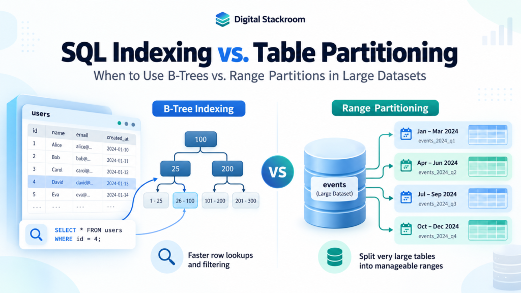
When queries begin to slow down on multi-million row tables, engineering teams often reach for the same immediate fix: add another index. While indexing solves row-level access bottlenecks, it is only one dimension of database performance.
As datasets scale beyond 50 million to 100 million rows, disk I/O and cache management become critical bottlenecks. Write amplification spikes, maintenance operations stall, and index trees grow too large to fit in RAM. This is the boundary where physical data placement—specifically table partitioning—becomes necessary alongside indexing.
Understanding the fundamental trade-offs between SQL indexing and table partitioning helps prevent memory bloat, high CPU usage, and sluggish query execution.
Table of Contents
1. Problem Statement & Real-World Use Case
Consider an e-commerce platform processing financial transactions (orders table). During its initial phase, a single relational table handles reads and writes seamlessly. However, after scaling to 80 million records, two issues typically emerge:
- Analytical Queries Degrade: Financial queries like
SELECT SUM(amount) FROM orders WHERE order_date >= '2026-01-01'trigger sequential scans over hundreds of gigabytes of disk space. - Buffer Cache Contention: A standard B-Tree index on
(order_date, customer_id)can grow past 15 GB. If the working memory (shared_buffers) cannot hold the full index alongside active data blocks, every lookup requires physical random disk I/O, degrading concurrent write and update speeds. - Data Purging Lockouts: Archiving obsolete records via
DELETE FROM orders WHERE order_date < '2023-01-01'locks rows, generates massive write-ahead log (WAL) volume, and produces dead tuple bloat that triggers aggressiveVACUUMlocks.
Solving this requires understanding what B-Tree indexes and partitions actually do at the storage layer.
2. Architecture & Mechanical Differences
┌────────────────────────────────────────────────────────┐
│                      SQL INDEX                         │
│  • Structure: Auxiliary B-Tree search structure        │
│  • Lookup Complexity: O(log N)                         │
│  • Best For: Point lookups and high-cardinality keys   │
│  • Storage: Lives in an auxiliary file alongside data  │
└────────────────────────────────────────────────────────┘

┌────────────────────────────────────────────────────────┐
│                  TABLE PARTITIONING                    │
│  • Structure: Physical segmentation into child tables  │
│  • Lookup Complexity: Linear boundary check O(P)       │
│  • Best For: Coarse data placement & partition pruning │
│  • Storage: Segregated physical files per boundary     │
└────────────────────────────────────────────────────────┘
The Mechanism of B-Tree Indexing
A standard SQL index does not change how data is organized on disk. Instead, it creates an auxiliary data structure (typically a balanced tree) containing the indexed column values and a pointer (such as a tuple ID / ctid in PostgreSQL) back to the heap page where the raw record lives.
- Selectivity is King: Indexes excel when a query targets a tiny fraction of the table (typically less than 2–5% of total rows).
- Write Overhead: Every
INSERT,UPDATE, orDELETErequires updating the B-Tree node pointers, leading to write latency and disk fragmentation over time.
The Mechanism of Table Partitioning
Table partitioning breaks one logical table into multiple physical child tables on disk. When a query with a filter runs, the query planner evaluates the boundaries of each partition and skips partitions that do not match the filter criteria—a mechanism known as Partition Pruning.
- Linear Data Reduction: While a B-Tree operates via logarithmic search $O(\log N)$, partitioning reduces search space in coarse segments.
- Zero-Downtime Data Lifecycles: Instead of running heavy
DELETEstatements, old data can be removed instantly using metadata operations likeDETACH PARTITIONorDROP TABLE.
3. Comparison Matrix
| Feature | SQL Indexing (e.g., B-Tree) | Table Partitioning (Range / List / Hash) |
| Primary Goal | Accelerates row-level lookups and sorting. | Manages data placement, segment pruning, and storage lifecycles. |
| Optimal Use Case | Point lookups (WHERE id = 58201) or high-cardinality filters. | Range queries on continuous keys (WHERE created_at BETWEEN X AND Y). |
| Write Penalty | High: Every write updates all associated index trees. | Low to Moderate: Engine routes write straight to the designated partition. |
| Storage Impact | Adds dedicated index disk overhead. | No redundant data overhead; uses standard storage pages. |
| Purging Old Data | Slow (DELETE produces WAL bloat and requires vacuuming). | Fast (ALTER TABLE DETACH PARTITION / DROP TABLE). |
| Memory Utilization | Cache thrashing when full index exceeds available RAM. | Only indexes of active partitions load into working memory. |
4. Practical Hands-On Implementation: PostgreSQL
Let’s compare an unpartitioned table with a range-partitioned implementation.
Step 1: Create an Unpartitioned Table and Benchmark
-- 1. Create standard table
CREATE TABLE orders_unpartitioned (
    order_id BIGSERIAL PRIMARY KEY,
    customer_id INT NOT NULL,
    order_date DATE NOT NULL,
    amount NUMERIC(10, 2) NOT NULL,
    status VARCHAR(20) NOT NULL
);

-- 2. Populate with 10 million test rows
INSERT INTO orders_unpartitioned (customer_id, order_date, amount, status)
SELECT
    (random() * 500000)::INT,
    '2024-01-01'::DATE + (random() * 730)::INT, -- Spans 2024-2025
    (random() * 1000)::NUMERIC(10, 2),
    (ARRAY['COMPLETED', 'PENDING', 'CANCELLED'])[floor(random() * 3 + 1)]
FROM generate_series(1, 10000000);

-- 3. Add standard B-tree index
CREATE INDEX idx_unpart_date ON orders_unpartitioned(order_date);
ANALYZE orders_unpartitioned;
Run an analytical aggregation query covering Q1 2024:
EXPLAIN ANALYZE
SELECT
    DATE_TRUNC('month', order_date) AS month,
    COUNT(*),
    SUM(amount)
FROM orders_unpartitioned
WHERE order_date BETWEEN '2024-01-01' AND '2024-03-31'
GROUP BY 1;
Execution Plan Analysis: The optimizer must balance whether to scan the idx_unpart_date index or perform a parallel sequential scan across all 10 million rows. Because 12.5% of the total dataset matches the filter, index lookups incur significant random I/O heap fetches, forcing the query engine into an expensive multi-worker scan across the entire heap file.
Step 2: Implement Range Partitioning with Local B-Tree Indexes
Set up declarative range partitioning on the identical dataset, chunked by calendar year:
-- 1. Create the parent partitioned table
-- Note: Partition key (order_date) must be part of the primary key constraint
CREATE TABLE orders_partitioned (
    order_id BIGINT GENERATED ALWAYS AS IDENTITY,
    customer_id INT NOT NULL,
    order_date DATE NOT NULL,
    amount NUMERIC(10, 2) NOT NULL,
    status VARCHAR(20) NOT NULL,
    PRIMARY KEY (order_id, order_date)
) PARTITION BY RANGE (order_date);

-- 2. Create physical range partitions
CREATE TABLE orders_y2024 PARTITION OF orders_partitioned
    FOR VALUES FROM ('2024-01-01') TO ('2025-01-01');

CREATE TABLE orders_y2025 PARTITION OF orders_partitioned
    FOR VALUES FROM ('2025-01-01') TO ('2026-01-01');

CREATE TABLE orders_default PARTITION OF orders_partitioned DEFAULT;

-- 3. Add local indexes across each partition automatically
CREATE INDEX idx_part_date ON orders_partitioned(order_date);
CREATE INDEX idx_part_cust ON orders_partitioned(customer_id);

-- 4. Load equivalent 10 million rows
INSERT INTO orders_partitioned (customer_id, order_date, amount, status)
SELECT customer_id, order_date, amount, status FROM orders_unpartitioned;

ANALYZE orders_partitioned;
Now execute the exact same aggregation query:
EXPLAIN ANALYZE
SELECT
    DATE_TRUNC('month', order_date) AS month,
    COUNT(*),
    SUM(amount)
FROM orders_partitioned
WHERE order_date BETWEEN '2024-01-01' AND '2024-03-31'
GROUP BY 1;
Execution Plan Analysis:
Append  (cost=0.43..12345.20 rows=1250000 width=48) (actual time=0.081..95.221 rows=3 loops=1)
  ->  Bitmap Heap Scan on orders_y2024 orders_partitioned_1
        Recheck Cond: ((order_date >= '2024-01-01'::date) AND (order_date <= '2024-03-31'::date))
        ->  Bitmap Index Scan on orders_y2024_order_date_idx
...
What changed?
- Partition Pruning: The query engine checked the metadata and excluded
orders_y2025andorders_defaultbefore touching disk. - Reduced Index Footprint: The index scan executed strictly against
orders_y2024_order_date_idx, which is half the size of the global index on the unpartitioned table. - Execution Speed: Query latency dropped significantly because 50% of the table’s total physical blocks were pruned before scanning began.
5. Architectural Edge Cases & Pitfalls
Pitfall 1: Over-Partitioning
Creating daily partitions for a table with low ingest rates creates hundreds of tiny physical relations. In PostgreSQL, each table and partition consumes file descriptors, locks, and catalog metadata. Over-partitioning slows down the query planner during plan generation and causes cache pressure on internal system catalogs.
Rule of thumb: Partitions should generally hold at least several gigabytes or millions of records each. If individual partitions hold under 100,000 rows, range partitioning adds unnecessary overhead.
Pitfall 2: Queries Omitting the Partition Key
If an application queries a partitioned table without specifying the partition key in its WHERE clause:
-- Missing order_date predicate
SELECT * FROM orders_partitioned WHERE customer_id = 98210;
The planner must scan every single child partition individually. While local indexes on customer_id will still be used, the execution plan executes an Append node over all partitions, adding minor overhead compared to querying a single unpartitioned table.
Pitfall 3: Unique Constraints & Primary Keys
In declarative partitioning, any PRIMARY KEY or UNIQUE constraint must include the partition column. You cannot enforce a global unique constraint on order_id alone across partitioned tables in PostgreSQL without including order_date.
6. Decision Tree: Which Strategy Should You Choose?
Is the total table size under 10–20 Million rows?
├── YES ───► Stick to targeted B-Tree / Partial Indexes (Partitioning adds unnecessary complexity).
└── NO  ───► Does the data have a natural range or time boundary (e.g., date, tenant ID)?
             ├── NO  ───► Optimize composite indexes, clustering, or evaluate sharding.
             └── YES ───► Combine Table Partitioning (coarse boundary elimination)
                          WITH Local B-Tree Indexes (fine row seek within partitions).
Indexes and partitioning are complementary rather than mutually exclusive. Range partitioning defines where physical chunks of data sit on disk, while B-Tree indexes provide point-lookup speed inside those individual partitions. Combining both allows large datasets to scale efficiently while keeping maintenance overhead low.